In this tutorial we will walk through each of the chunking strategies supported by DocParse and provide examples of how to use them.

Context-Rich

The context rich chunking strategy combines adjacent elements with one another and adds the last seen section header or title to each outputted chunk. For example, let’s take the fifth page of the following document:
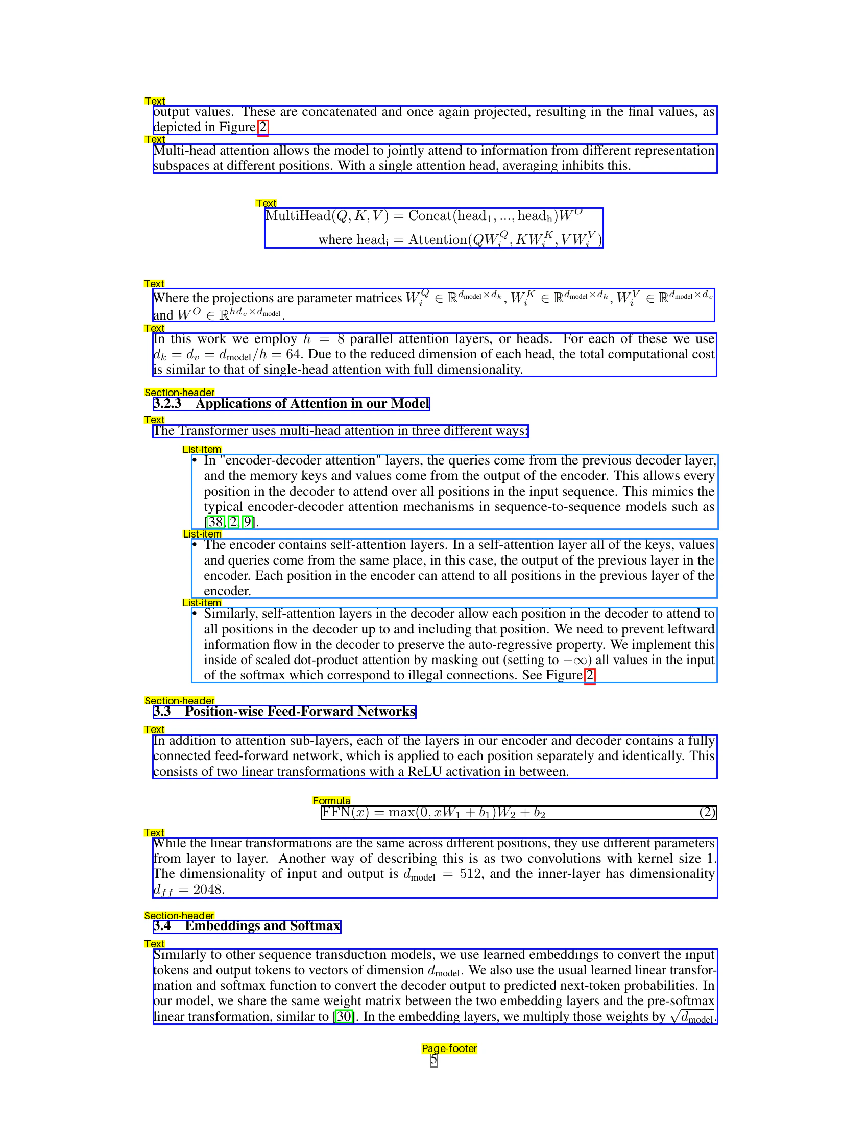
The bounding boxes shown above are the result of calling DocParse without any chunking options specified. Let’s say for your question/answering RAG application, you want to easily be able to retrieve certain formulas and ask questions such as “What linear transforms were used for Position-wise Feed-Forward Networks?” This would require the Section Header “Position-wise Feed-Forward Networks,” to be in the same chunk as the Formula (2) “FFN(x)=…”. Calling DocParse with the following chunking options will group the two chunks together:

chunking_options={
  "strategy": "context_rich",
  "tokenizer": "openai_tokenizer",
  "tokenizer_options": {
    "model_name": "text-embedding-3-small"
  },
  "merge_across_pages": True,
  "max_tokens": 512,
}

with open("transformers.pdf", "rb") as f:
  data = partition_file(f, aryn_api_key, chunking_options=chunking_options)
  

If you inspect the elements in the return value, you’ll notice that the Section Header and the Formula are all chunked together into one element:

{
  "properties": {
    "score": 0.9430291056632996,
    "page_number": 5,
    "page_numbers": [
      5
    ]
  },
  "type": "Text",
  "binary_representation": null,
  "text_representation": "**3.3 Position-wise Feed-Forward Networks**\n\nIn addition to attention sub-layers, each of the layers in our encoder and decoder contains a fully\nconnected feed-forward network, which is applied to each position separately and identically. This\nconsists of two linear transformations with a ReLU activation in between.\n\n **FFN(x) = max(0, xW1 + b1)W2 + b2**\n (2)\n\nWhile the linear transformations are the same across different positions, they use different parameters\nfrom layer to layer. Another way of describing this is as two convolutions with kernel size 1.\nThe dimensionality of input and output is dmodel = 512, and the inner-layer has dimensionality\ndf f = 2048.\n",
  "bbox": [
    0.17546135397518384,
    0.6537761896306818,
    0.8272261316636029,
    0.8000078790838068
  ],
  "_header": "3.3 Position-wise Feed-Forward Networks\n"
}

Maximize Within Limit

The maximize_within_limit strategy is meant to be used when you want to merge several consecutive elements together into a large chunk. Take the following example:
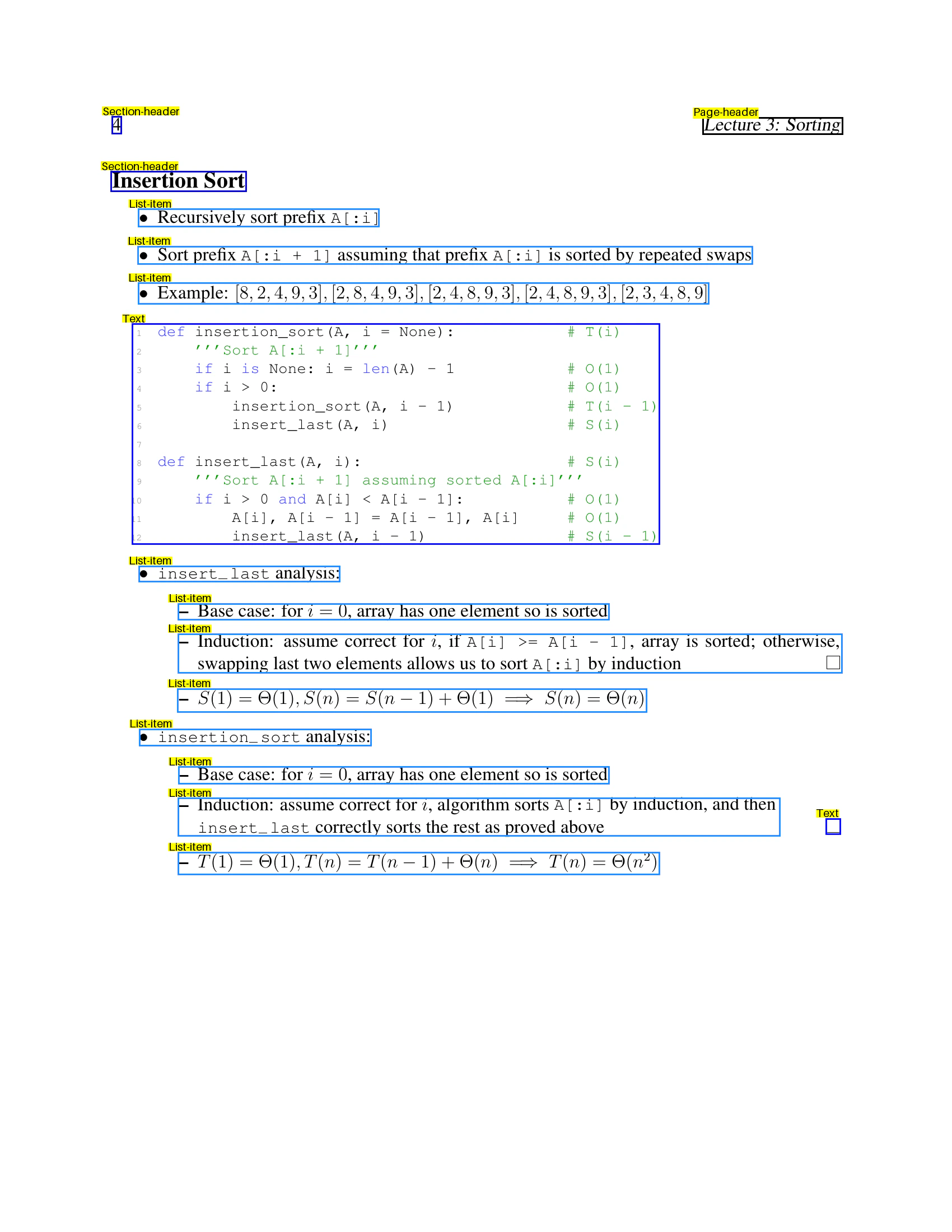
The bounding boxes shown above are the result of calling DocParse without any chunking options specified. Let’s say for your question/answering RAG application, you want all the list items to be grouped together into one chunk to improve the quality of your embeddings. Calling DocParse with the following chunking options will group the entire list into one chunk:

chunking_options={
  "strategy": "maximize_within_limit",
  "tokenizer": "openai_tokenizer",
  "tokenizer_options": {
    "model_name": "text-embedding-3-small"
  },
  "merge_across_pages": True,
  "max_tokens": 512,
}

with open("transformers.pdf", "rb") as f:
  data = partition_file(f, aryn_api_key, chunking_options=chunking_options)

If you inspect the elements list in the return value, you’ll notice that the entire bulleted list in the document is grouped into one chunk:


{
    "properties": {
        "score": 0.5081191062927246,
        "page_number": 4,
        "page_numbers": [
            4
        ]
    },
    "type": "Section",
    "binary_representation": null,
    "text_representation": "4 \n\nLecture 3: Sorting \n\nInsertion Sort \n\n\u2022  Recursively sort pre\ufb01x A[:i] \n\n\u2022  Sort pre\ufb01x A[:i  +  1] assuming that pre\ufb01x A[:i] is sorted by repeated swaps \n\n\u2022  Example: [8, 2, 4, 9, 3], [2, 8, 4, 9, 3], [2, 4, 8, 9, 3], [2, 4, 8, 9, 3], [2, 3, 4, 8, 9] \n\n1  def  insertion_sort(A,  i  =  None): \n\u2019\u2019\u2019Sort  A[:i  +  1]\u2019\u2019\u2019 \n2 \nif i is None: i = len(A) - 1 \nif i > 0: \n 3 \n 4 \n 5 \n 6 \n insertion_sort(A,  i  - 1) \ninsert_last(A,  i) \n 7 \n8  def  insert_last(A,  i): \n9 \n \u2019\u2019\u2019Sort  A[:i  +  1]  assuming  sorted  A[:i]\u2019\u2019\u2019 \nif i > 0 and A[i] < A[i - 1]: \n A[i],  A[i  - 1]  =  A[i  - 1],  A[i] \ninsert_last(A,  i  - 1) \n 10 \n 11 \n 12 \n #  T(i) \n # O(1) \n# O(1) \n#  T(i  - 1) \n#  S(i) \n #  S(i) \n # O(1) \n#  O(1) \n#  S(i  - 1) \n\n\u2022  insert  last analysis: \n\n\u2013  Base case: for i = 0, array has one element so is sorted \n\n\u2013  Induction:  assume correct for i,  if  A[i]  >=  A[i  - 1],  array is sorted;  otherwise, \n swapping last two elements allows us to sort A[:i] by induction \n\n\u2013  S(1) = \u0398(1), S(n) = S(n \u2212 1) + \u0398(1)  =\u21d2  S(n) = \u0398(n) \n\n\u2022  insertion  sort analysis: \n\n\u2013  Base case: for i = 0, array has one element so is sorted \n\n\u2013  Induction: assume correct for i, algorithm sorts A[:i] by induction, and then \n insert  last correctly sorts the rest as proved above \n\n\u2013  T (1) = \u0398(1), T (n) = T (n \u2212 1) + \u0398(n) =\u21d2  T (n) = \u0398(n2) \n",
    "bbox": [
        0.11637571447035845,
        0.09453096563165839,
        0.8855567842371324,
        0.7101616876775568
    ]
}